Neuron differentiation case study
stoic_neuron_differentiation.Rmd
library(stoic)Use case
In this vignette, stoic will be used on a systems biology case study, to extract meaningful associations between:
- Transcriptional activity profiles of regulatory regions (enhancers or promoters) in the course of neuron differentiation
- The DNA sequence features within those regions. Here, we use the frequency of k-mers. Other sequence features could be considered, like transcription factor binding motif scores.
This single cell dataset (sampled here, and not public yet) was generated as part of a collaboration within the FANTOM6 project, in the lab of Chi Wai Yip (RIKEN).
The methodology of STOIC allows to find groups of co-expressed regulatory regions that can be well discriminated by sequence features. It does so through an exploration of the expression space where co-expression clusters are formed by maximizing the classification performance of predicting cluster membership based on sequence features.
Such a guidance of clustering by sequence information has the advantage to discover stronger associations between the two modalities, and only focus on clusters predictable by sequence.
This approach could be generalized to any question where the clustering of observations in one type of data can be informed by another type of data, and where the user wants to learn the associations between the two.
Data import
We start by creating the data used by stoic. It needs two matrices:
The main data matrix, giving, for each observation, values in a set of samples. In our case this is, for 1000 regulatory regions, the transcriptional activity in 391 cellular states ordered along neuron differentiation (metacells). We recommend using several hundreds or even thousands of observations in stoic, and several tenths or hundreds of samples.
The guide data matrix, that gives, for each observation, a set of complementary features used to inform clustering. In our case study this is the sequence characteristics of 1000 regulatory regions, i.e k-mers frequencies with from 1 to 3. We recommend several tenths or thousands of guide features in stoic.
(Optional) The order of the samples in the main data, for visualization purposes only. In our case, this is the numerical metacell order during neuron differentiation. It can be numeric or alphanumeric.
data("neuron_diff")
data <- stoic_data(main_data = neuron_diff$main_data,
           guide_data = neuron_diff$guide_data,
           sample_order = neuron_diff$sample_order, seed = 666)
Running stoic
The guided clustering procedure can then be launched by stoic. Below
is an example with two different initializations (nstart,
as in kmeans), which are later combined to take the best clusters. We
recommend increasing nstart for even more stable results (e.g 5 or
more).
The classification model in stoic is a Random Forest, of which the number of trees can be set.
stoic_results <- stoic_clustering(data, nstart = 2, n_cores = 4, n_trees = 500, seed = 666)
table(stoic_results$clusters)
#>
#>    1    2    3    4    5 none
#>   27   94   17  315   36  511
The results contain several objects in a list, the most important being:
-
clusters: a named vector that gives cluster membership to all observations (a number, or “none” if no cluster was found in the area of this observation). -
aucs: a named vector that gives the AUC (classification performance) for each cluster. -
best: a list of all clusters learned by stoic, containing more details like the list of observations, AUC, the model and its predictions, the important guide features, the correlation threshold and centroid of the cluster, and so on.
Most notably, we can access the sequence feature importance of a given cluster (number 2 here) as follows:
head(get_feature_importance(stoic_results, 2))
#>   feature  importance importance_min importance_max direction
#> 1      CA 0.004745341    0.004310244    0.005180438      TRUE
#> 2      CG 0.004040024    0.003541362    0.004538686     FALSE
#> 3     GCA 0.003418567    0.003009708    0.003827426      TRUE
#> 4     CCG 0.002469698    0.002083054    0.002856342     FALSE
#> 5     CGA 0.002211791    0.001850673    0.002572910     FALSE
#> 6      CC 0.001807957    0.001502072    0.002113841     FALSE
The direction column is TRUE when the feature has higher values in the cluster than in other observations, FALSE otherwise.
Visualization of the results
A few visualization solutions are included in the package, and are assembled together below. This gives an overview of the clustering, by showing the observations in the main space (the expression space, reduced in a tSNE), and colored by cluster. Next to it, the activity profiles of the regulatory regions appear for each cluster, ranked by AUC. Stoic here identified a series of diverse expression profiles during the differentiation process (like activation, repression, peaks in intermediary states, …).
draw_tsne(data, stoic_results) +
  draw_profiles(data, stoic_results)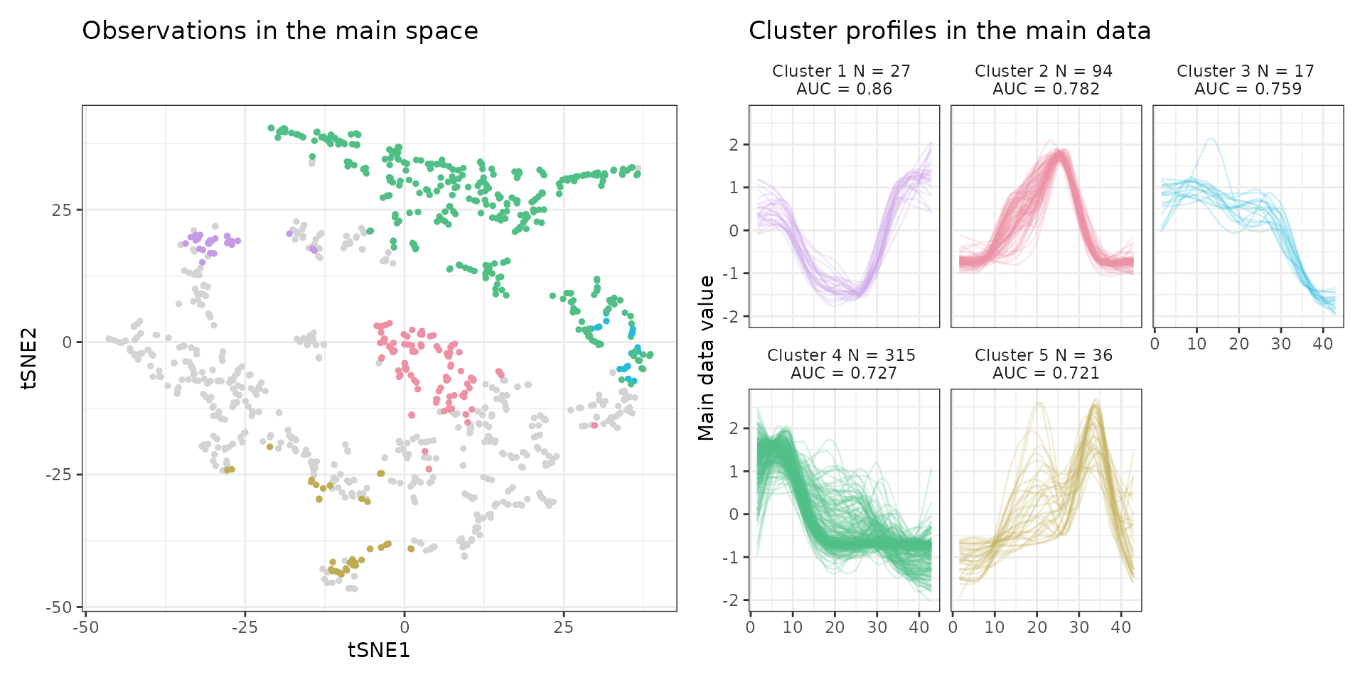
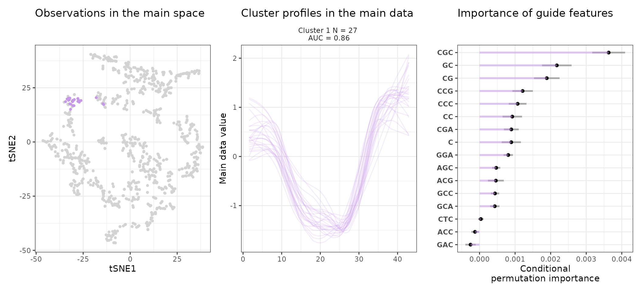
One can also look at a given cluster of interest, as in the following lines, where the important sequence features for the cluster also appear.
for (i in 1:length(stoic_results$best)){
  print(
    draw_tsne(data, stoic_results, cluster = i) +
  draw_profiles(data, stoic_results, cluster = i) +
  draw_features(data, stoic_results, cluster = i, only_positive = T,
                n_top_features = 20)
  )
}
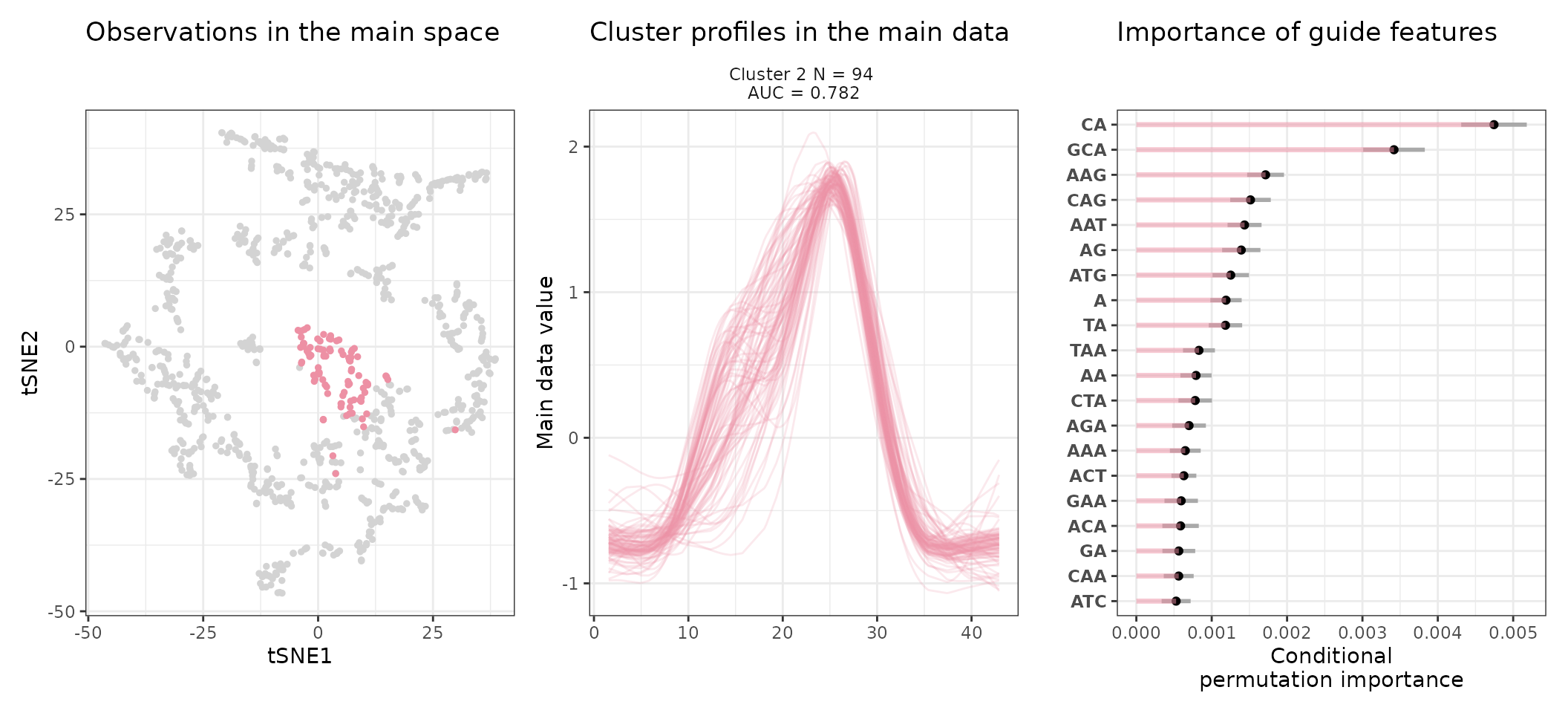
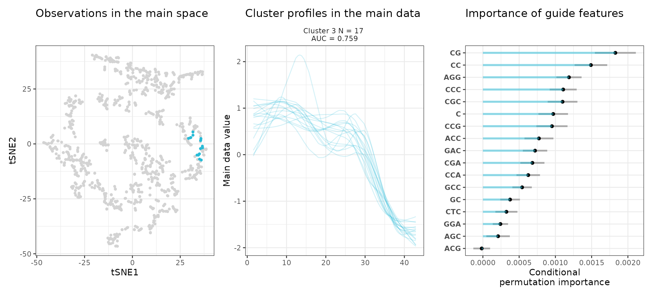
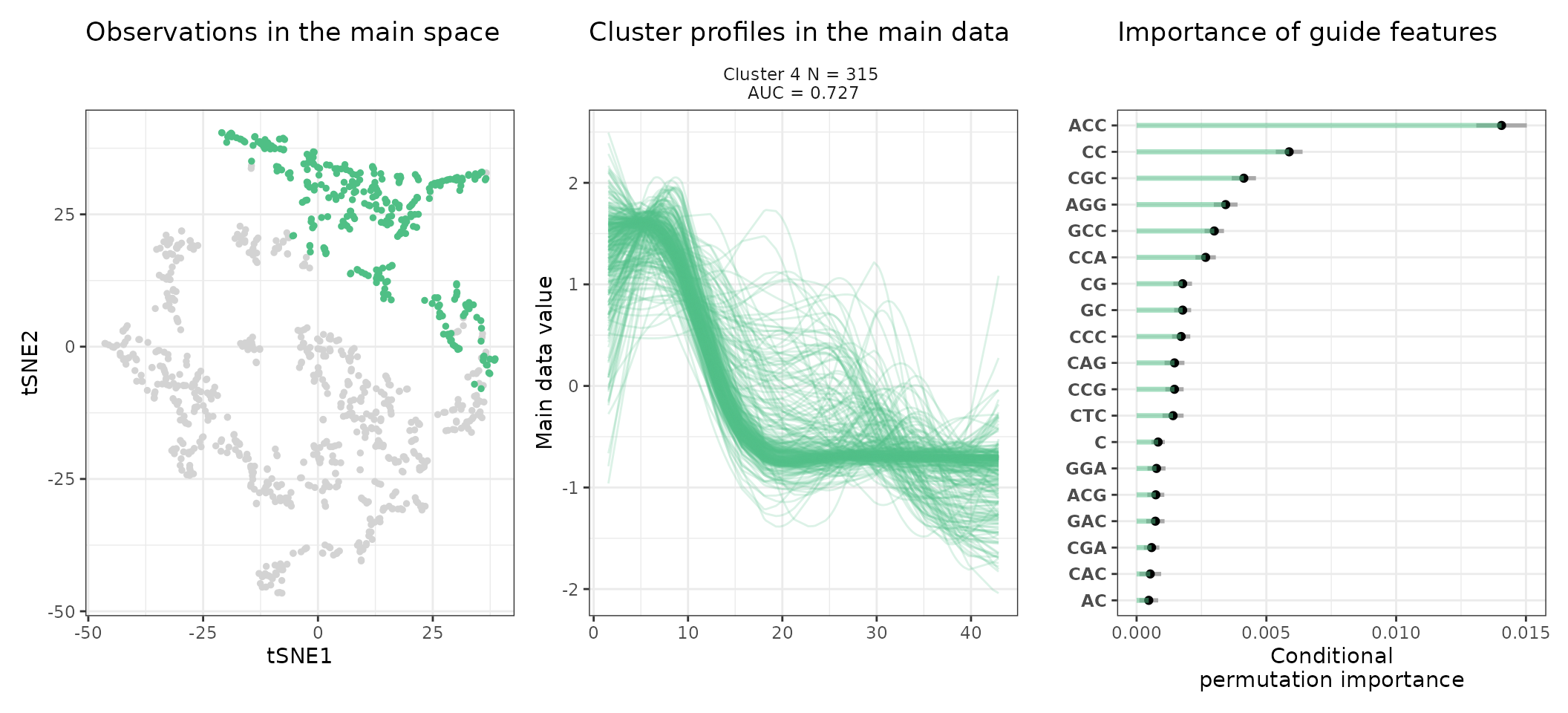
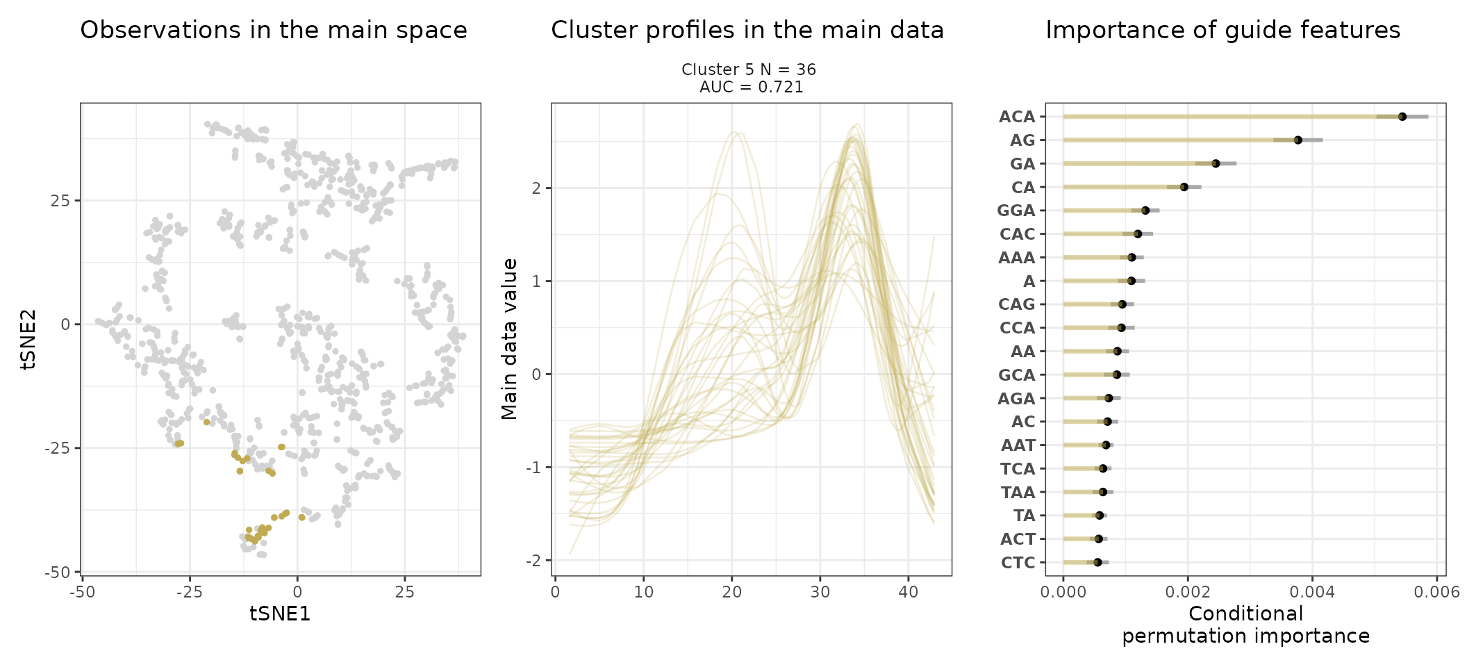
An interpretation of cluster 2 based on stoic results would be: “This set of 93 enhancers and promoters are mostly active and transcribed in the middle of the differentiation process (neural stem cells), and can be characterized in terms of sequence by A-rich k-mers such as CA or AAG. Sequence features, combined together, allow to discriminate these regulatory regions from others transcriptionnally variable regions with an AUC of 0.78”
Similarity of stoic clusters
It can also be helpful to see how similar are the inferred clusters to one another. This is done internally by stoic to prune redundant clusters, but can also be visualized downstream of the clustering. Three similarity measures are used:
A symmetrical swap score (between 0 and 1), where the model of one cluster is used to predict the membership of another cluster. It tells us weather or not the rules learned from the guide data (sequence features) are the same (score = 1), or similar (score close to 1), between two clusters.
The linear correlation of the profile in the main data (expression here), between two clusters.
The Jaccard index (overlap/union) between two clusters (the real positive classes of the clusters are considered, before the final step of assigning observations to one cluster only).
draw_clusters_similarity(data, stoic_results)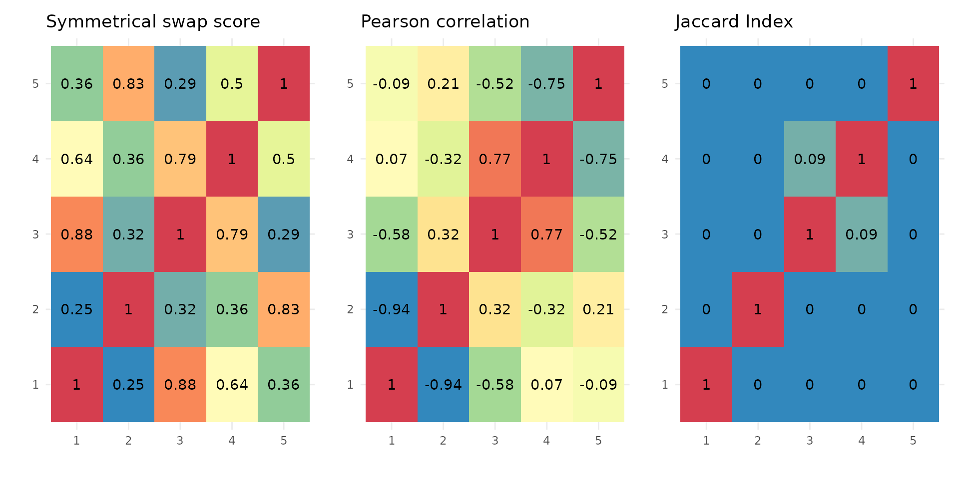
This can help the user interpret clusters, but also potentially tune
the swap threshold score used in the stoic_clustering
function. Clusters are deemed redundant if their swap score is above the
swap threshold supplied (0.95 by default), if their Jaccard index is not
0, and if they are correlated over the maximum correlation threshold
learned to define the two clusters.
Vizualize sequence features within a cluster
Stoic provides a heatmap function to show the scores of the important
sequence features within a cluster (selected via an elbow rule), and
compare them to observations outside a cluster. The obs
parameters allow to chose whether we want to show only the observations
within the cluster, outside the cluster, or all observations with an
annotation about cluster information.
For example, in the first cluster:
draw_features_heatmap(stoic_results, data, cluster = 1, obs = "cluster")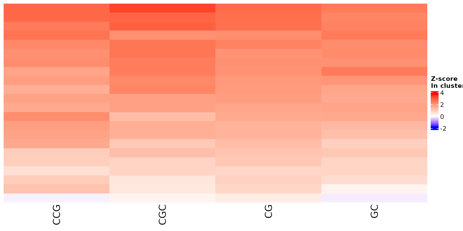
draw_features_heatmap(stoic_results, data, cluster = 1, obs = "other")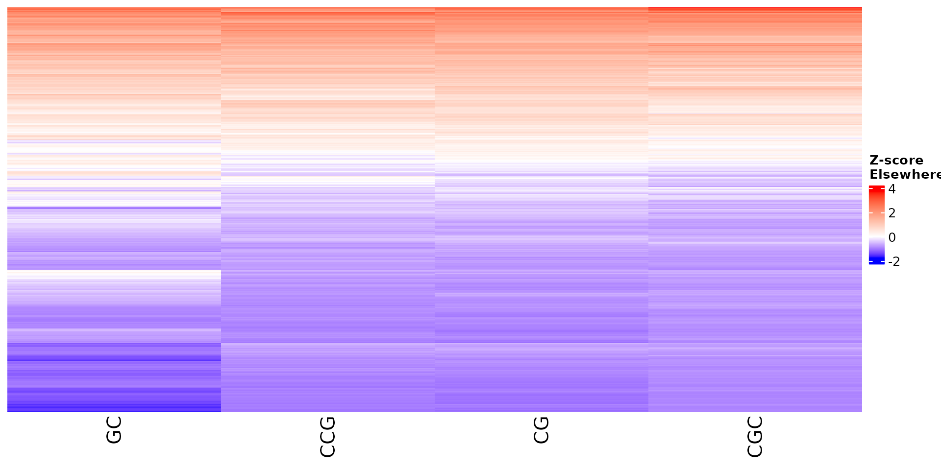
draw_features_heatmap(stoic_results, data, cluster = 1, obs = "all")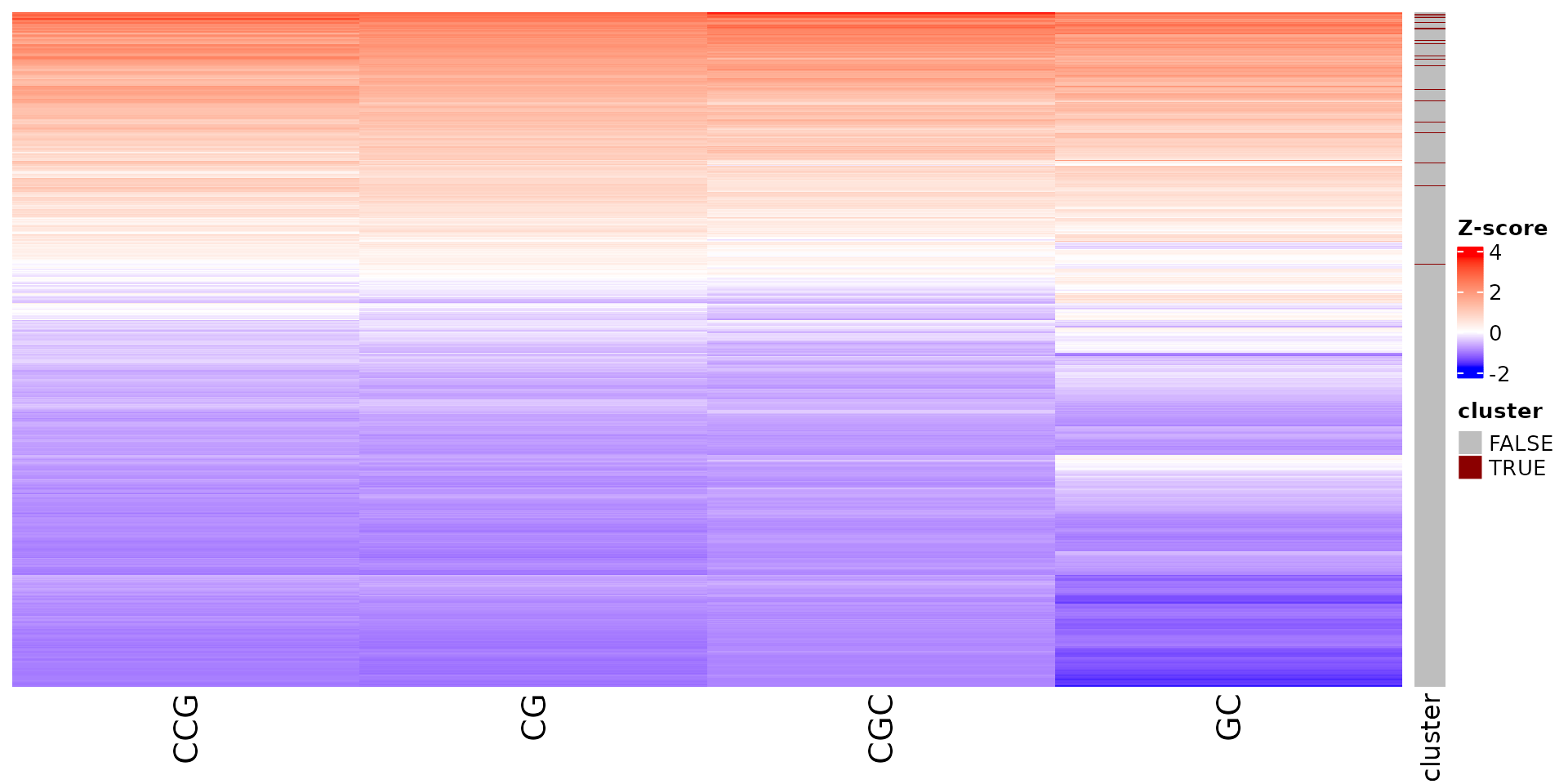
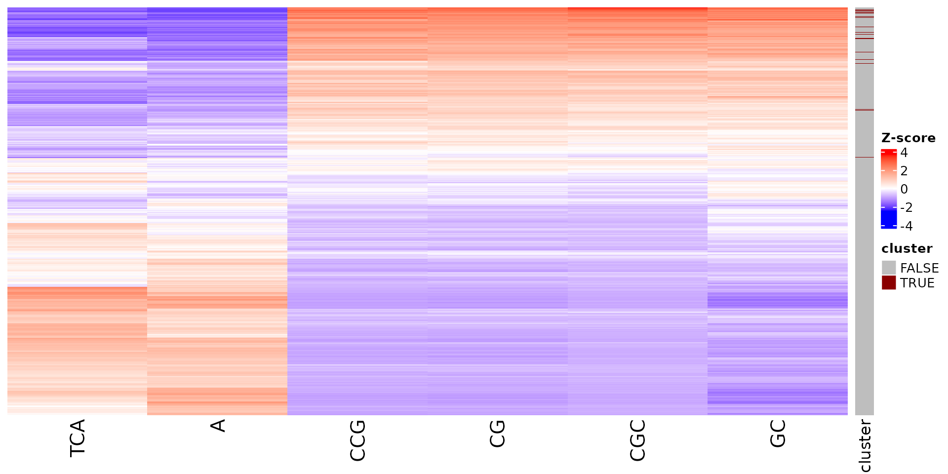
All sequence features are scaled to a z-score within all observations, so red values indicate higher than average values, and blue lower than average. By default, only the important sequence features enriched in the cluster are shown, but all important features including depleted ones can also be shown as follows:
draw_features_heatmap(stoic_results, data, cluster = 1, obs = "cluster", only_positive = F)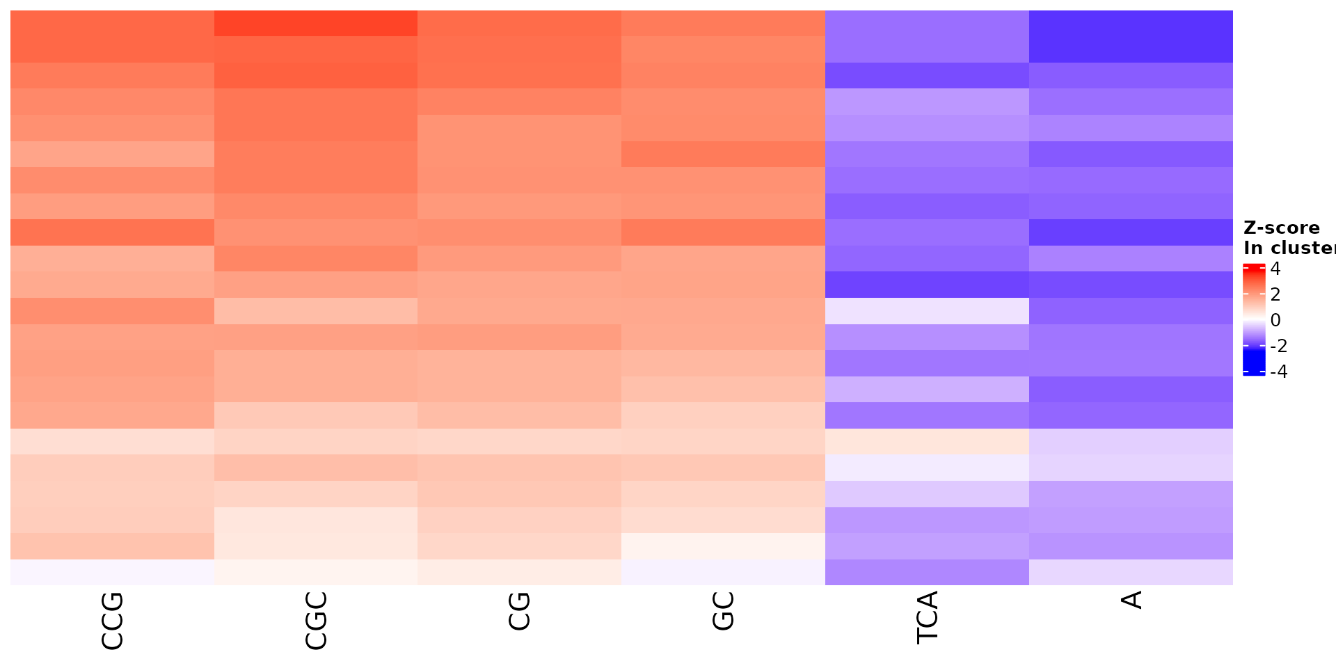
draw_features_heatmap(stoic_results, data, cluster = 1, obs = "other", only_positive = F)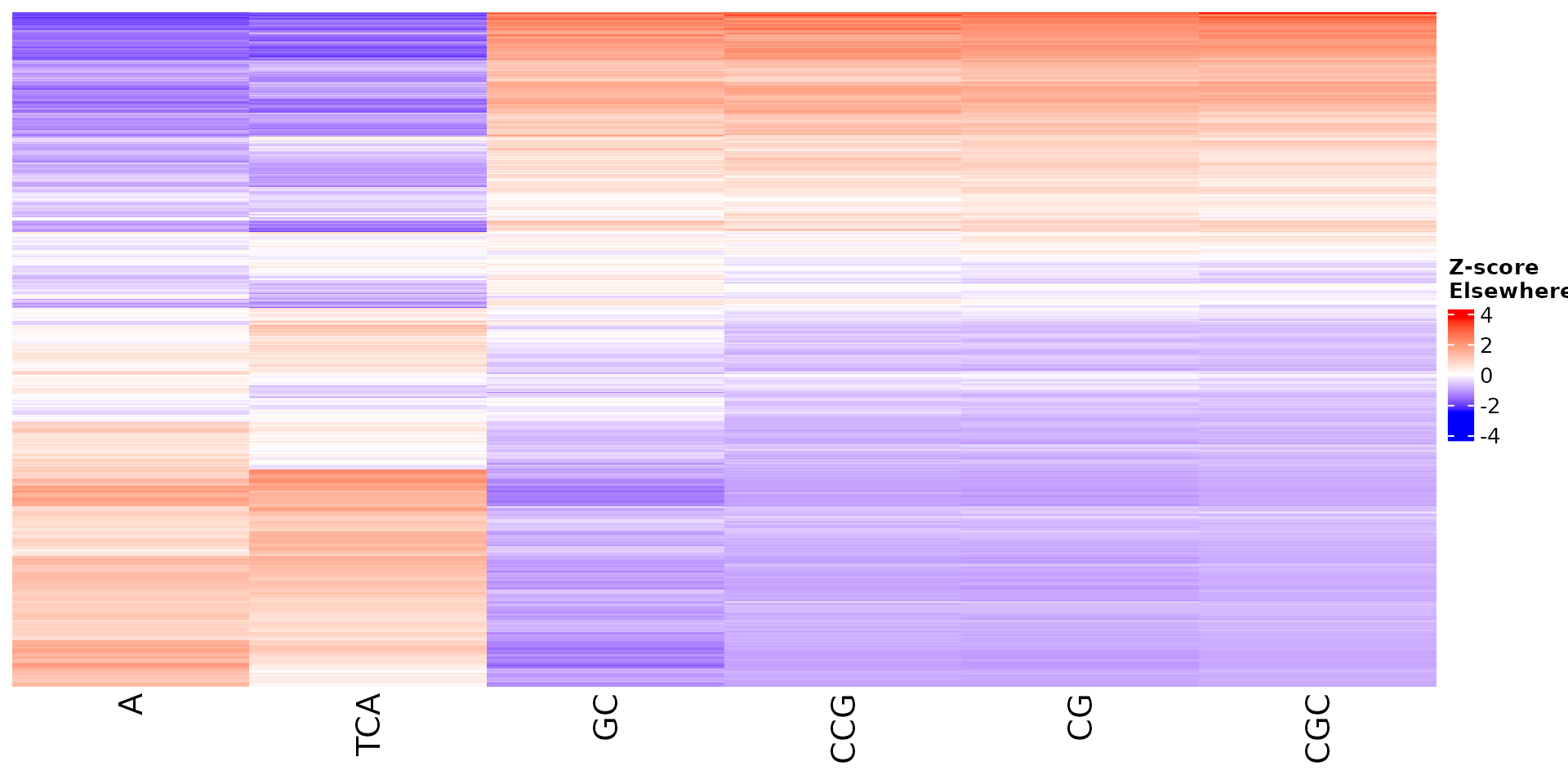
draw_features_heatmap(stoic_results, data, cluster = 1, obs = "all", only_positive = F)